Time complexity and scaling
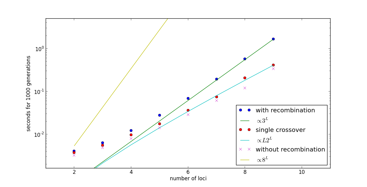
Recombination is implemented in haploid_lowd in such a way that it scales with the number of loci as \(\mathcal{O}(3^L)\) instead of the naive \(\mathcal{O}(8^L)\). Moreover, if a single crossover event is allowed to happen, the complexity is reduced even further to \(\mathcal{O}(L\, \cdot 2^L)\). This is shown in this example, called speed_lowd.py.
First, modules and paths are imported as usual, plus the time module is imported as well:
import time
Second, population parameters are set:
N = 1000                        # Population size
Lmax = 12                        # Maimal number of loci
r = 0.01                        # Recombination rate
mu = 0.001                      # Mutation rate
G = 1000                        # Generations
Third, simulations of G generations are repeated for various number of loci L, to show the scaling behaviour of the recombination algorithm:
exec_time = []
for L in range(2,Lmax):
    t1=time.time()
    ### set up
    pop = h.haploid_lowd(L)     # produce an instance of haploid_lowd with L loci
    pop.carrying_capacity = N   # set the population size

    # set and additive fitness function. Note that FFPopSim models fitness landscape
    pop.set_fitness_additive(0.01*np.random.randn(L))

    pop.set_recombination_rates(r)  # assign the recombination rates
    pop.set_mutation_rates(mu)  # assign the mutation rate

    #initialize the population with N individuals with genotypes 0, that is ----
    pop.set_allele_frequencies(0.2*np.ones(L), N)

    pop.evolve(G)               # run for G generations

    t2=time.time()

    exec_time.append([L, t2-t1])    # store the execution time

exec_time=np.array(exec_time)
Fourth, the same schedule is repeated with a simpler recombination model, in which only one crossover is allowed, setting the recombination rates with the optional argument pop.set_recombination_rates(r, h.SINGLE_CROSSOVER), and without recombination, using haploid_lowd.evolve_norec instead of the haploid_lowd.evolve.
Fifth, the time required is plotted agains the number of loci and compared to the expectation \(\mathcal{O}(3^L)\):
plt.figure()
plt.plot(exec_time[:,0], exec_time[:,1],label='with recombination', linestyle='None', marker = 'o')
plt.plot(exec_time[:,0], exec_time[-1,1]/3.0**(Lmax-exec_time[:,0]-1),label=r'$\propto 3^L$')

plt.plot(exec_time_norec[:,0], exec_time_norec[:,1],label='without recombination', linestyle='None', marker = 'x')
plt.plot(exec_time[:,0], exec_time_norec[-1,1]/2.0**(Lmax-exec_time_norec[:,0]-1),label=r'$\propto 2^L$')

plt.plot(exec_time[:,0], exec_time[-1,1]/3.0**(Lmax)*8**(exec_time[:,0]),label=r'$\propto 8^L$')

ax=plt.gca()
ax.set_yscale('log')
plt.xlabel('number of loci')
plt.ylabel('seconds for '+str(G)+' generations')
plt.legend(loc=2)
plt.xlim([1,Lmax])
plt.ylim([0.2*np.min(exec_time_norec[:,1]),10*np.max(exec_time[:,1])])

plt.ion()
plt.show()
The result confirm the theoretical expectation: